Anatomy of BoltzGen

A comprehensive exploration of BoltzGen's architecture: from molecular representations to diffusion-based generation of protein binders
A comprehensive exploration of BoltzGen's architecture: from molecular representations to diffusion-based generation of protein binders
We have entered the era of generative biology. While tools like AlphaFold solved the problem of predicting how nature folds proteins, the frontier has shifted to designing novel molecules that nature never evolved: proteins that can bind to specific targets, neutralize pathogens, or catalyze new reactions.
Unlike previous approaches that often simplified proteins to their backbones, BoltzGen is an all-atom diffusion model capable of "co-folding" binders and targets simultaneously.
It extends beyond just proteins, integrating DNA, RNA, and small molecules into a single, unified generative framework. But how does a neural network hallucinate a physically valid, atomic-level 3D structure from pure noise? In this article, we will tear apart the architecture to understand the machinery under the hood.
If you, like me, have mostly an ML background, you may be used to thinking in terms of inputs and outputs and how we can effectively represent them for a task. In order to do so, we have to take a quick detour and learn the basics of the domain we are dealing with. In our case, the output goal is to generate binders (proteins or peptides) given as input a biomolecular target (other proteins, small molecules, DNA/RNA) and some specified conditions.
Let's not be afraid of all this terminology. Learning in detail about all these entities might require you to follow an entire biochem curriculum, but I am going to try to introduce the bare minimum to make some sense of this.
Both proteins and peptides are fundamentally chains of the same basic units called amino acids, which are
essentially small organic molecules.
All amino acids share a fundamental structure built around a central carbon atom known as the alpha-carbon
(α-carbon). This central carbon is bonded to four different groups:

While all amino acids share the same first three groups, what characterizes their chemical properties is the
structure of the side chain, that varies for each one of them.
In order to form a chain, these aminoacids bind in a dehydration process (losing an H2O molecule). We call
shorter chains (usually between 2 and 50 aminoacids) peptides, while longer chains are called proteins.
Each unit of a chain is called a residue, and has two main parts:
Currently, we can formulate a preliminary hypothesis on how to encode this information. It would look really tempting to express a chain the same way we express a sentence: a sequence of tokens! Could we just get away with defining something like:
# tripeptide glycylhistidyllysine (Gly-His-Lys residues sequence)
tripeptide = ["GLY","HIS","LYS"]
and then let the model train on a next token prediction task?
Right now, we are actually missing another key information that we need to model from this data: these are not simple sequences of residues, but each of the atoms making up those residues has a particular position in 3D space. Modelling this is of fundamental importance because the binding process is something that occurs in physical space, where the geometry of both binder and target is essential.
Now that we've established the dual nature of our problem (continuous 3D coordinates and discrete amino acid labels), we face a challenge: how do we treat this duality in a single model? The solution is the 14 atoms representation.
Here's how it works: Each residue is represented by 14 atoms, the length of the longest possible residue. The first 4 are always the backbone atoms (N, Cα, C, O), while the remaining 10 are "virtual atoms" that act as markers. The model signals which amino acid it wants by placing a specific number of these virtual atoms directly onto the backbone atoms. We then decode the amino acid identity by counting how many virtual atoms land on each backbone position (within 0.5 Å).
For example: threonine is signaled by placing 3 virtual atoms on the backbone nitrogen and 4 on the backbone oxygen. Proline uses 7 atoms on the oxygen. Glycine uses 10 on the oxygen. The remaining atoms that aren't used as markers become the actual side chain.
This clever encoding lets the model work entirely in continuous 3D space, avoiding the messy problem of mixing discrete and continuous representations. It enables efficient joint training for both structure prediction and sequence design. To see this in action, I prepared a minimal example from the original codebase in this notebook.
Recalling what we introduced at the beginning, we are interested in designing binders that interact with some defined target. BoltzGen allows for non-designed inputs that can be proteins (or protein sequences), nucleic acids (DNA/RNA) and small molecules. Being an all-atom model, we can pass detailed atomic level information such as atom positions, element types and charge.
Raw information for these entities is tipically stored in PDB or mmCIF formats. Let's take a look at an example description of a small protein chain in PDB format:
ATOM      1  N   GLY A   1      25.864  33.665  -2.618 ... N
ATOM      2  CA  GLY A   1      26.039  32.227  -2.528 ... C
ATOM      3  C   GLY A   1      27.247  31.766  -3.284 ... C
ATOM      4  O   GLY A   1      27.359  32.164  -4.437 ... O
ATOM      5  N   ALA A   2      28.140  30.984  -2.678 ... N
ATOM      6  CA  ALA A   2      29.336  30.435  -3.271 ... C
ATOM      7  C   ALA A   2      30.455  31.439  -3.133 ... C
ATOM      8  O   ALA A   2      30.334  32.498  -3.611 ... O
ATOM      9  CB  ALA A   2      29.623  29.088  -2.639 ... C
...
Taking a look at this we can see that a chain is described as a long list of atoms. Let's break down what we're seeing:
ATOM: Tells us this is an atom record.CA, N, C, CB: These are the specific atom names
(e.g., Carbon-alpha, Nitrogen).GLY, ALA: These are the residue (or "token") names (Glycine, Alanine).A: This is the chain ID.1, 2: These are the residue (token) numbers.25.864 33.665 -2.618: These are the X, Y, and Z coordinates in 3D space.N, C, O: The element type.Once we have defined our inputs and their nature, it's finally time to talk about machine learning. The first piece we need is an encoder, which in BoltzGen is defined as the trunk. The trunk module is responsible of creating embeddings for designed and non designed inputs, together with conditioning specifications. Within the trunk, we have a multi-stage encoding approach that aims at extracting meaningful information at different levels. Let's now see how it works in detail.
When studying a certain molecule, we can derive meaningful information at different scales, from the individual atomic level to the interaction between residues. It makes sense then, to design an encoder that tries to extrapolate information in a hierarchical way.

In BoltzGen, inputs are handled by an Input Embedder model, which is made up by two core modules: an atom encoder, and an atom attention encoder.
The Atom Encoder takes the raw features for each atom and return two types of output: single atom
# Compute raw input embedding
q, c, p, to_keys = self.atom_encoder(feats)
# Project pairwise features
atom_enc_bias = self.atom_enc_proj_z(p)
After deriving representations at the atomic level, it's time to go up in the hierarchy and model th interaction between residues. This operation is done in two stages by the Atom Attention Encoder. Here we have two stages:
# a are the token embeddings from the attention encoder
a, _, _, _ = self.atom_attention_encoder(
    feats=feats,
    q=q,
    c=c,
    atom_enc_bias=atom_enc_bias,
    to_keys=to_keys,
)
We already discussed that the generation procedure can be conditioned on a number of different specifications. We can steer generation specifying:
The conditioning process in the trunk is fairly simple, and is computed only at the initial stage. All of the
specs are embedded either using nn.Embeddings modules or linear layers. Once embedded, this
information is added to the token embeddings
# condition the token embeddings
s = (
    a
    + self.res_type_encoding(res_type)
    + self.msa_profile_encoding(torch.cat([profile, deletion_mean], dim=-1))
)

if self.add_method_conditioning:
    s = s + self.method_conditioning_init(feats["method_feature"])
# ... sum of all other possible conditionsLet's make a small recap. At this stage we computed token-level embeddings
This is a two stage process, where we first initialize pairwise features
As a first step, starting from our token embeddings, we build a pairwise feature matrix
As you can see, after applying the outer sum we create a matrix where for each entry
We now go a step further, trying to add to this representation some geometric and topological information for each pair. This operation is done by adding to the pairwise feature matrix relative position encodings derived from the featurs. At this stage we add information about:
Now we proceed adding information by deriving a bynary adjacency matrix token_bonds , where the
entry token_bonds[i,j] is 1 if tokens
This adds information about bond type (single, double, triple, aromatic, etc.) via an embedding layer.
In order to steer conditional generation, the user is allowed to enforce specific distances between two residues, and say if these residues should be in either of these three states:
This information is computed using Fourier embeddings and added to our pairwise feature matrix.
The following image show schematically the initialization of pairwise features, starting from individual
token embeddings, to pairwise matrix creation and conditioning to get to the feature matrix

As you might have noticed, we are slowly building up representations at increasingly higher levels of abstractions. We started from single atoms to tokens, and got to pairs of tokens. What we are still missing at this point is trying to build a more complete 3D-aware understanding of these relationships. The initial pairwise feature matrix is not enough to capture this, as it only blindly looks at pairs of tokens.
For this reason we use a pairformer module, whose job is to take this basic information and build a sophisticated, geometrically-aware understanding of the entire molecular complex. This is done by trying to iteratively enforce the respect of the triangle inequality.
Let's try to make an example to explain this rule: if I told you that city A is distant 10km from city B, and city B is distant 10km to city C, would you believe that the distance from A to C is 100km?

Well, the short answer is no because of the simple reason that the shortest path between two points is always a straight line: the distance between A and C cannot be longer tha the distance from C to A passing by B.
The problem right now is that our pairwise feature matrix might represent incorrect information that does not respect this property, because we only looked at pairs of tokens.
My second question for you now is: why should we care about ensuring that this inequality is satisfied among the triplets in our representations?
Because the triangle is the smallest, simplest polygon. It's the bare minimum unit needed to introduce spatial logic. What we expect is that by respecting this rule for all triplets, we are able to compositionally get a whole 3D geometric structure representation that actually makes sense.
Let's now get to how the Pairformer works, but first I just want to show you a picture that represents how a triplet can be seen from a pairwise matrix perspective and a graph one.
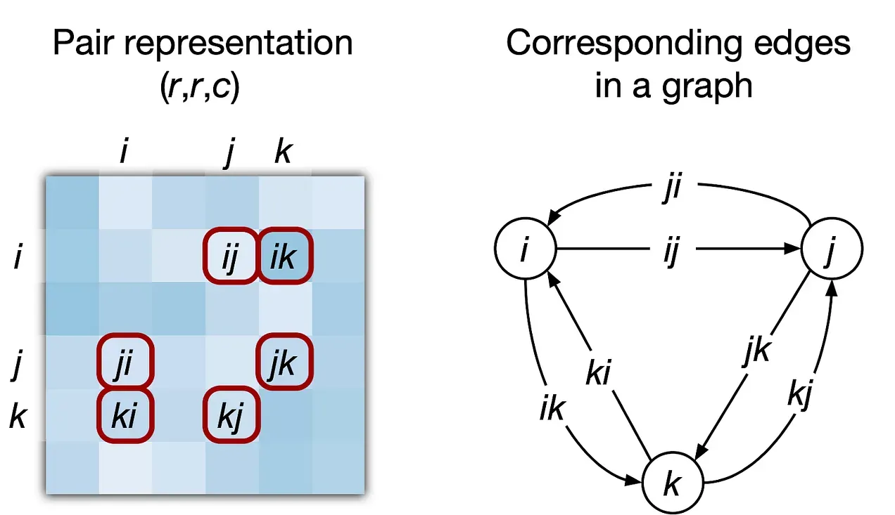
Notice that for each pair of nodes
What the Pairformer does is apply a stack of "reasoning layers". Each layer in this stack has two main jobs.
First, it updates the pairwise matrix

Second, it updates the single token representations
This whole two-part process (updating pairs, then updating tokens) forms one single Pairformer layer. This block is stacked on top of itself multiple times, allowing the model to iteratively refine its understanding of the 3D geometry until it represents a physically plausible structure.
We have now established a complete overview of the processing performed by the trunk. This module encodes physical and context-aware features, transforming raw atomic data into rich token embeddings and pairwise representations.
Operating at this atomic level enables the model to unify a diverse range of input modalities within a single framework. These extracted features serve as the critical conditioning signal used to steer the generative diffusion process, which we're going to discuss in the next section.
Let's now get to the core functionality of BoltzGen, which is designing proteins and peptides that bind to given biomolecular targets. The generative process is based on the paradigm of diffusion models, where our model starts from purely noisy atomic coordinates and will try to iteratively denoise them until we get to a final generated structure.
While the most traditional approaches are based on docking (given a binder structure, predict the target), one of the most notable points of this generation process is that our model is trained on a co-folding task. This means that we are trying to make the model generate both the structure of the target and the binder at the same time.
The key insight is that by forcing the model to reason about sequence and structure together at every step, the resulting designs are more likely to be physically coherent and plausible. Moreover, the model should learn to capture all-atom interactions: this is critical because it allows the model to learn how the sequence (which determines the sidechains) can influence the backbone structure, and vice-versa.
As we already discussed, the generation process is driven by a diffusion module. I will not go to deep in explaining how diffusion models work in general, as there are plenty of already good resources (I really like this video by Depth First). In this section I'd rather describe how the standard diffusion process has been adapted for our molecular generation task.
What happens at a high level is that our model, starting from pure noisy atomic coordinates for both the target and the binder learn to reconstruct both structures at the same time via a multi-step denoising process, which is steered by all the meaningful information that has been embedded by the trunk.

Mathematically, given a sample expressed as 3D atomic coordinates from our training data:
We increasingly add noise for
The goal of our denoiser module

At each denoising steps, sampling from the denoiser is done by following the EDM framework proposed by Karras et al. where at each step, before sampling from a denoiser, we add a bit of randmom noise to the previous sample.
This may sound counterintuitive, but it's one of the key parts for improving the quality of our generation. This kind of "shake" that we give to our denoising trajectory helps with two things: trying to bump back on the correct path if the model starts going towards an incorrect route, and most of all encouraging our model to explore diverse protein structures.
This procedure is regulated by two scaling factors:
This is another clever trick implemented in the model generation phase, which comes from an observation of the authors: the most critical part of the design happens between 60% and 80% of the denoising process. Within this window, the model makes the actual design decision of the amino acid type for each residue.
The natural consequence was to dilate the time in this window. This means that if we defined a number of
denoising steps
With the model's architecture fully defined, we can now summarize the operational workflow. BoltzGen takes a fixed target and a conditional binder as inputs, encoding them into rich, property-aware structural embeddings. In the subsequent design phase, the process begins with a vector of atom coordinates initialized as random noise. The model then iteratively denoises this vector, using the condition embeddings as a guide to progressively reveal the final binder structure.
Now that we have seen the various parts that compose the model, it's time to talk about how it's trained. As we discussed, we want the model to learn how to behave given a diverse set of conditions.
To achieve this, the model isn't just trained on one specific problem (like only predicting a structure), but on a mixture of different tasks and conditions all at once.
This "jack-of-all-trades" approach is what makes BoltzGen a universal model. During training, the pipeline randomly samples a known biomolecular structure from its database, crops it, and then "pretends" parts of it are unknown. This setup can create several different types of problems for the model to solve.
The model learns its versatility by being randomly assigned one of several key tasks for each training example. The main tasks include:
By constantly switching between these tasks, BoltzGen learns the fundamental rules of protein physics, folding, and interaction simultaneously, all within a single model.
On top of the general task, the model is also trained to obey a rich set of specific conditions. This is what gives the user precise control over the final output. During training, these conditions are randomly applied to the known structures:
The loss used in BoltzGen training is used to ensure our model learns to reconstruct the correct molecular structure at different scales, and takes the name of diffusion objective.
The diffusion objective computes measures on the structure of the prediction with respect to the ground
truth. Let's start by defining our denoiser's prediction as
The first measure we compute is the Mean Squared Error between the model's predicted atomic coordinates and the true ones:
This is a fairly standard measure, but we have to put the focus on two things. First, before computing the
MSE, a rigid alignment algorithm is applied to find the optimal transformation that matches
at best both structures. The reason for this is that since we're in 3D, our model might predict the correct
structure, but rotated with respect to the ground truth. This is why we create an
Second, we apply a weight
The second component of our diffusion objective is the Bond Loss. Here we encourage the model to generate correct bond lengths. For all the pairs of atoms that are bonded in the ground truth, we compare their distance with the distance in the predicted structure. This ensures the local atomic geometry is chemically correct:
Third and last component is the Smooth lDDT Loss. While before we focused on individual bond distances, now we try to check if the local environment around each atom is correct. We define a certain region cutoff and check all distances between neighbors in that region. We call it smooth because it gives partial credit (being 0.6 Å off is penalized less than being off 4.1 Å):
Where
The final formulation of our diffusion objective is:
Notice how here we have a weighting for MSE and bond loss
We have seen that BoltzGen was structured to work on a wide possible set of inputs and conditions. A key usability feature of the design process is the Design Specification Language, which allows the user to tell the model exactly what we want to design, what's the target and which rules to follow. This file follows the YAML convention, where we define entities and constraints. Let's now break down a couple of examples from the paper:
Our goal here is to design a small, cyclic peptide (between 8 and 18 residues long) that binds to the specific chain A of the protein streptavidin.
Notice how here we are adding even more specs than just residue length and binding site. This example shows also how we can characterize parts of the input. In this case we are saying that our target has a flexible group, meaning that our model will take into account this and generate a better fitting binder and simultaneously predicting how the target will adapt.
Although BoltzGen is the core for the generation of candidate designs, it can be considered a part of a pipeline that serves as a funnel that uses a series of increasingly rigorous computational checks to filter them down to a small, diverse, and high-quality set of candidates ready for expensive and time-consuming wet-lab validation.
The whole BoltzGen pipeline is a 6 steps process, that we will now look in detail:
BoltzGen pipeline represents a significant shift from isolated generative models to a comprehensive, end-to-end framework for biomolecular design. By integrating a powerful all-atom generative model with a rigorous filtering and ranking system, BoltzGen bridges the gap between computational generation and real-world applicability. Its ability to design across diverse modalities (from nanobodies to cyclic peptides) and its success in targeting novel proteins demonstrate its potential as a general-purpose tool for drug discovery.
BoltzGen represents a significant leap forward in the field of generative biology. Through extensive wet-lab validation (achieving success rates as high as 80% on complex targets) it has demonstrated how all-atom diffusion models can effectively design binders across a diverse set of modalities, including proteins, nucleic acids, and small molecules. Furthermore, by releasing the model and its comprehensive filtering pipeline as open source, the project empowers researchers globally to democratize access to these advanced tools, fostering a collaborative environment that accelerates the pace of discovery..
However, we are far from considering drug design a solved problem. While we now possess the capability to computationally generate thousands of promising candidates in a quick and integrated pipeline, the bottleneck has shifted to the laborious and costly phase of downstream validation. The rigorous demands of clinical trials remain a significant hurdle that must be cleared to translate designs into therapies. There is immense potential for artificial intelligence to bridge this gap, specifically through technologies like virtual cells and predictive modeling for clinical outcomes, which could drastically reduce the time and cost of bringing a drug to market.
Finally, there remains substantial room for the architectural optimization of these models. As detailed in the technical specifications, BoltzGen currently relies on a heavy "trunk" architecture for complex multi-level feature extraction, employing intricate components like PairFormer stacks and triangular attention mechanisms. This approach is now being challenged by emerging models like SimpleFold, which aim for simpler, general-purpose backbones. This tension raises a critical question for the future of the field: are we witnessing another instance of the "bitter lesson," where simpler, scalable architectures will eventually supersede complex, domain-specific engineering?
In short, BoltzGen shows what is possible today, but also highlights the vast landscape of challenges that remain. Improving controllability, accelerating downstream validation, simplifying the architecture, and better integrating predictive models of biological function will all be crucial steps toward making AI-driven drug design not just powerful, but practical.
I would like to thank @mozzarellapesto and @tensorqt for the friendly help in the review process.